— July 25, 2021
Visualizing Algorithm Runtimes in Python
Use code to visualize and determine runtime complexities for different algorithms.
This article will cover how you can use visualization libraries and software to determine runtime complexities for different algorithms. We will cover the basic usage of matplotlib for visualization of 2d plots and numpy for calculating lines of best fit, and then go over how these libraries can be used to determine their runtime complexity either through "guesstimation" or by comparing the plots of their runtimes to that of known functions (i.e. y=x, y=2^x).
If you are interested in downloading the code featured in this article, please visit this repository on my GitHub (chroline/visualizingRuntimes).
What is runtime complexity?
Runtime complexity, more specifically runtime complexity analysis, is a measurement of how “fast” an algorithm can run as the amount of operations it requires increases. Before we dive into visualizing the runtimes of different algorithms, let’s look at a couple of basic examples to explain the concept.
Take the following add function. It accepts two parameters, a and b, and performs addition on a and b.
1
2
def add(a, b):
    return a + b
When given any two parameters (1 and 2, 2 and 3, 29347 and 93648), the amount of operations does not change. Therefore, we say the algorithm runs in constant, or O(1) , time.
However, now consider the following permutations function. It accepts one main parameter, string, and prints all of the permutations of that string.
1
2
3
4
5
6
7
def permutations(string, step = 0):
    if step == len(string):
        print "".join(string)
     for i in range(step, len(string)):
        string_copy = [c for c in string]
        string_copy[step], string_copy[i] =string_copy[i], string_copy[step]
        permutations(string_copy, step + 1)
As you could imagine, this function would take much longer than the previous add function; in fact, this function would run in what is called factorial time, represented as O(n!). That is because as the amount of characters in string increases, the amount of operations required to find all the permutations increases factorially.
When comparing the runtimes of two functions visually, you would notice a stark contrast in the graphs they produce. For the add function, you would observe a flat line, as the input of the function does not affect the amount of operations required by the function. However, for the permutations function, you would observe a line that drastically spikes upwards (the slope of the line would approach infinity) because the amount of operations increases factorially as the size of the input increases.
Now that we have covered the basics of runtime complexity analysis, we can begin the process of writing code to visualize the runtimes of different algorithms.
Initialization
Before running any visualizations, we must first import the necessary libraries and initialize them.
matplotlibis a library that will create and display the graphs
numpyis a library that consists of numerous mathematical utility functions
timeitis a library that we will use to time how long each call to the algorithm takes
mathis the basic Python math library
randomis the basic Python randomization library
1
2
3
4
5
6
7
import matplotlib.pyplot as plt
import numpy as np
import timeit
import math
import random

plt.rcParams['figure.figsize'] = [10, 6] # set size of plot
Demos
Below are some code segments that demonstrate how to use matplotlib and numpy.
sum function
The Python sum function calculates the sum of all elements of a provided Iterable. This function implements an algorithm with a O(n) runtime complexity.
To test this, we will use the linspace method from the numpy library to generate an iterable with 50 evenly-spaced values ranging from 10 to 10,000. The graph, although not a perfectly straight plot, illustrates this.
1
2
3
4
5
ns = np.linspace(10, 10_000, 50, dtype=int)
ts = [timeit.timeit('sum(range({}))'.format(n), number=100)
      for n in ns]

plt.plot(ns, ts, 'or')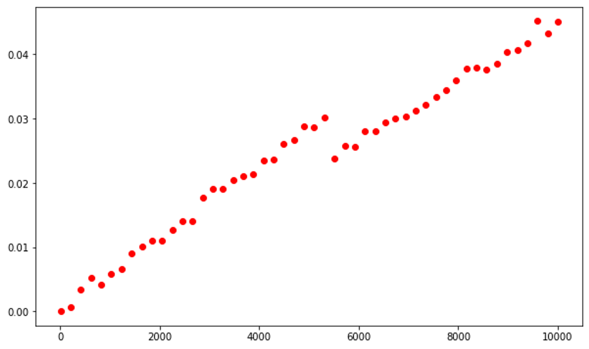
We can add a line of best fit (using a 4th-degree function) to further exemplify this. The graph will never be a perfectly straight-line, but it should come close.
1
2
3
4
5
degree = 4
coeffs = np.polyfit(ns, ts, degree)
p = np.poly1d(coeffs)
plt.plot(ns, ts,'or')
plt.plot(ns, [p(n)for nin ns],'-b')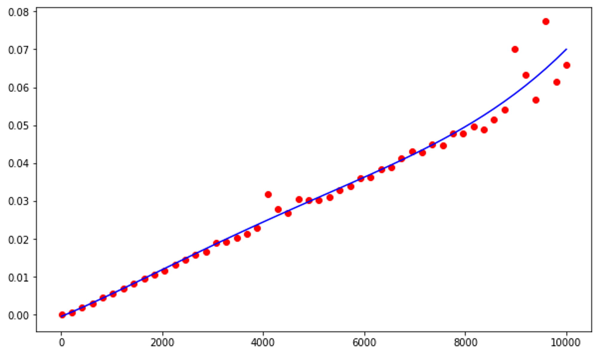
List Indexing
Retrieving an item from a list (list indexing) runs with O(1) runtime complexity, which means that the amount of items in the list does not affect how long the algorithm takes to run. How is this represented in a graph?
1
2
3
4
5
6
7
8
9
10
11
12
13
lst = list(range(1_000_000))
ns = np.linspace(0, len(lst), 1000, endpoint=False, dtype=int)
ts = [timeit.timeit('_ = lst[{}]'.format(n),
                    globals=globals(),
                    number=10000)
for nin ns]

plt.plot(ns, ts,'or')

degree = 4
coeffs = np.polyfit(ns, ts, degree)
p = np.poly1d(coeffs)
plt.plot(ns, [p(n)for nin ns],'-b')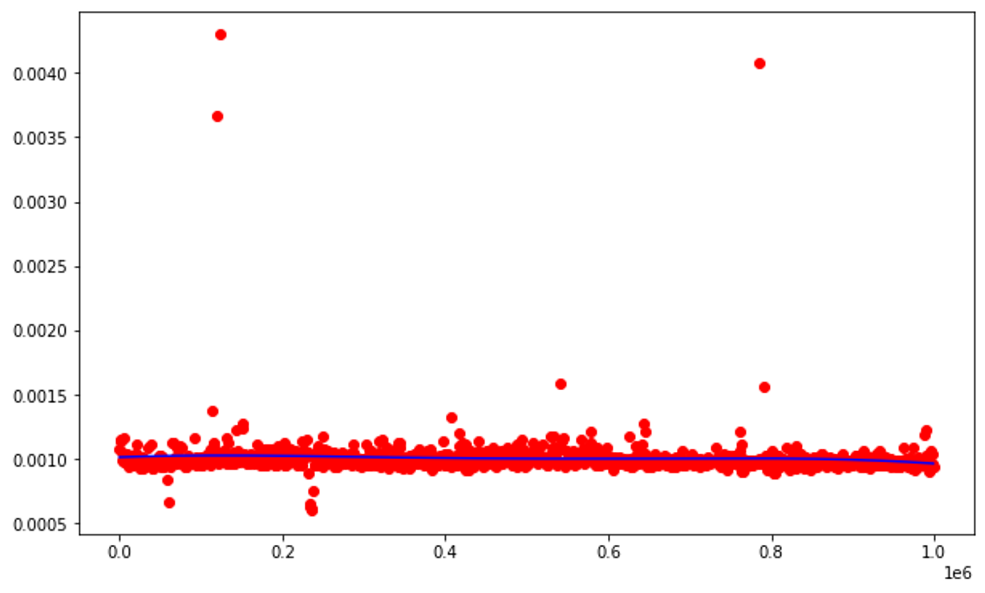
Algorithms
Now we will look at the graphs produced by the following algorithms:
- linear search
- binary search
- insertion sort
Linear Search
Linear search has a runtime complexity of O(n), which will be represented by an approximately straight line.
Red plots demonstrate searching for an element in a shuffled, blue plots demonstrate searching for an element that is not present in the list.
The line of best fit for the red plots will generally be lesser than that of the blue plots because searching for an element that is not present in the list requires iterating through the entire list.
1
2
3
4
5
6
7
8
9
10
11
12
13
14
15
16
17
18
19
20
21
22
23
24
25
26
27
28
29
30
31
32
33
34
35
## searches for an item in a list
def contains(lst, x):
    for y in lst:
        if x == y: return True
    return False

ns = np.linspace(10, 10_000, 100, dtype=int)

# red plots
ts = [timeit.timeit('contains(lst, 0)',
                    setup='lst=list(range({})); random.shuffle(lst)'.format(n),
                    globals=globals(),
                    number=100)
      for n in ns]
plt.plot(ns, ts, 'or')

# line of best fit for red plots
degree = 4
coeffs = np.polyfit(ns, ts, degree)
p = np.poly1d(coeffs)
plt.plot(ns, [p(n) for n in ns], '-r')

# blue plots
ts = [timeit.timeit('contains(lst, -1)',
                    setup='lst=list(range({}))'.format(n),
                    globals=globals(),
                    number=100)
      for n in ns]
plt.plot(ns, ts, 'ob')

# line of best fit for blue plots
degree = 4
coeffs = np.polyfit(ns, ts, degree)
p = np.poly1d(coeffs)
plt.plot(ns, [p(n) for n in ns], '-b')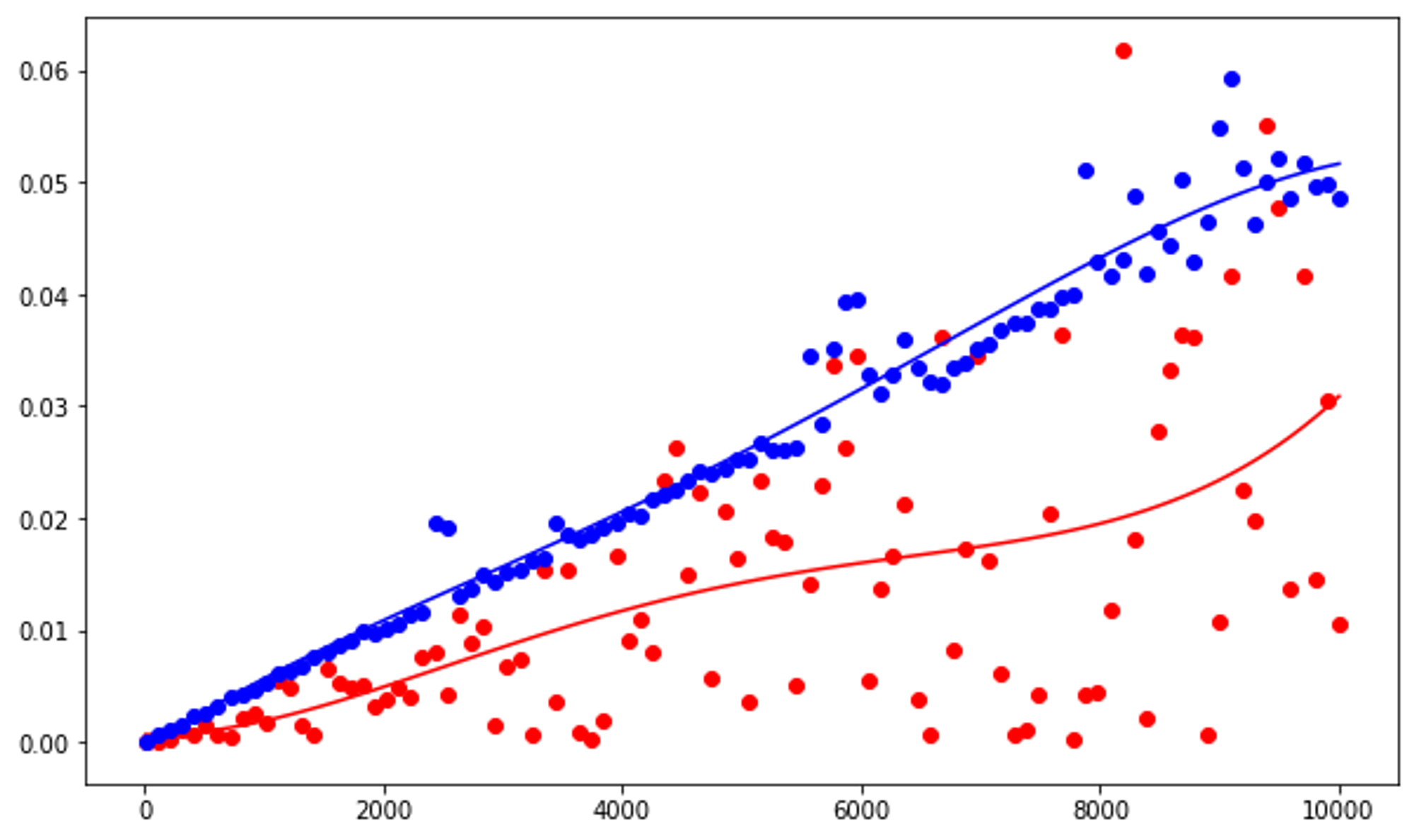
Binary Search
Binary search runs with O(log n) runtime complexity.
1
2
3
4
5
6
7
8
9
10
11
12
13
14
15
16
17
18
19
20
21
22
23
24
25
26
27
28
# searches for an item in a list using linear search
def contains(lst, x):
    lo = 0
    hi = len(lst)-1
    while lo <= hi:
        mid = (lo + hi) // 2
        if x < lst[mid]:
            hi = mid - 1
        elif x > lst[mid]:
            lo = mid + 1
        else:
            return True
    else:
        return False

ns = np.linspace(10, 10_000, 100, dtype=int)
ts = [timeit.timeit('contains(lst, 0)',
                    setup='lst=list(range({}))'.format(n),
                    globals=globals(),
                    number=1000)
      for n in ns]

plt.plot(ns, ts, 'or')

degree = 4
coeffs = np.polyfit(ns, ts, degree)
p = np.poly1d(coeffs)
plt.plot(ns, [p(n) for n in ns], '-b')
Above is what the graph should look like in a near-perfect simulation. As you can see, there are some some outliers, and in a perfect simulation the line of best fit would be identical to a logarithmic function.
Insertion Sort
What runtime complexity does insertion sort have? We can use the plots of its runtime and compare those plots against the graphs of known runtimes to determine which is the closest match.
1
2
3
4
5
6
7
8
9
10
11
12
13
14
15
16
17
18
19
20
21
def insertion_sort(lst):
    for i in range(1, len(lst)):
        for j in range(i, 0, -1):
            if lst[j-1] > lst[j]:
                lst[j-1], lst[j] = lst[j], lst[j-1]
            else:
                break

# 15 values
ns = np.linspace(100, 2000, 15, dtype=int)
ts = [timeit.timeit('insertion_sort(lst)',
                    setup='lst=list(range({})); random.shuffle(lst)'.format(n),
                    globals=globals(),
                    number=1)
         for n in ns]
plt.plot(ns, ts, 'or');

degree = 4
coeffs = np.polyfit(ns, ts, degree)
p = np.poly1d(coeffs)
plt.plot(ns, [p(n) for n in ns], '-r')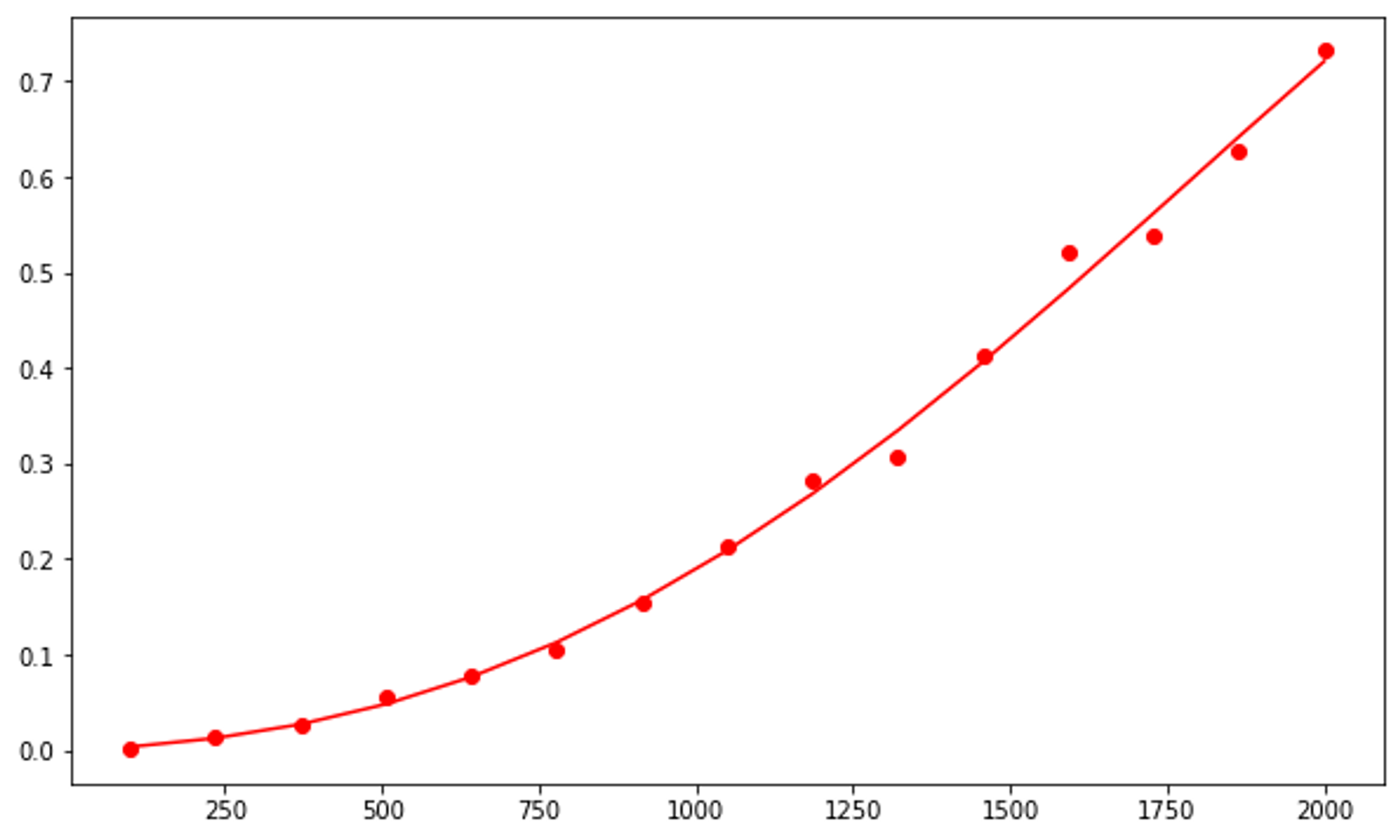
Now, we can compare that graph with graphs of different runtimes to ultimately determine which is most similar and which runtime complexity insertion sort has.
Red plots represent O(log n), blue plots represent O(n^2), green plots represent O(2^n)
1
2
3
4
5
6
7
8
9
10
11
12
13
14
15
16
17
18
# y = log x
# vertically stretched 1000x
ns = range(1, 100)
ts = [math.log(n, 2) * 1000 for n in ns]
plt.plot(ns, ts, 'or');

# y = x^2
ns = range(1, 100)
ts = [(n*n) for n in ns]
plt.plot(ns, ts, 'ob');


# y = 2^x
# vertically stretched 20x
# horizontally compressed 1x
ns = range(1, 10)
ts = [math.pow(2, n)*20 for n in ns]
plt.plot(ns, ts, 'og');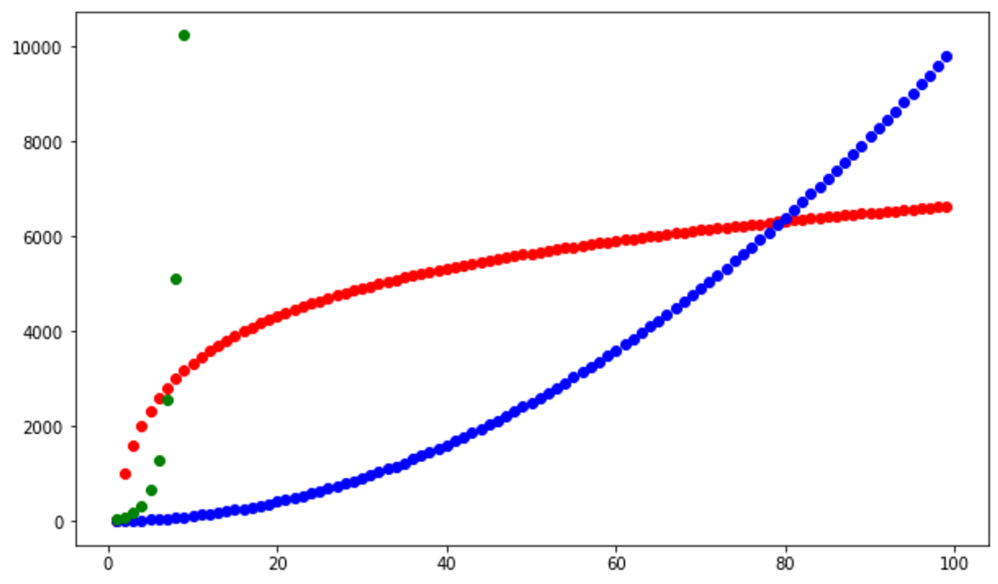
Based on these graphs, it is safe to assume that insertion sort runs in O(n^2) time.
Mystery function runtime analysis
Can we use visualization of the runtimes of mystery functions to guesstimate their runtime complexities?
Mystery function #1
1
2
3
4
5
6
7
8
9
10
11
12
13
14
15
16
17
18
def f(l: list, val): # l is a python list with n items
  d = {}
  for i in range(len(l)):
    d[l[i]] = i
  return d[val]

ns = range(5, 2000)
ts = [timeit.timeit('f(lst, {})'.format(n-1),
                    setup='lst=list(range({})); random.shuffle(lst)'.format(n),
                    globals=globals(),
                    number=1)
         for n in ns]
plt.plot(ns, ts, 'or');

degree = 4
coeffs = np.polyfit(ns, ts, degree)
p = np.poly1d(coeffs)
plt.plot(ns, [p(n) for n in ns], '-b')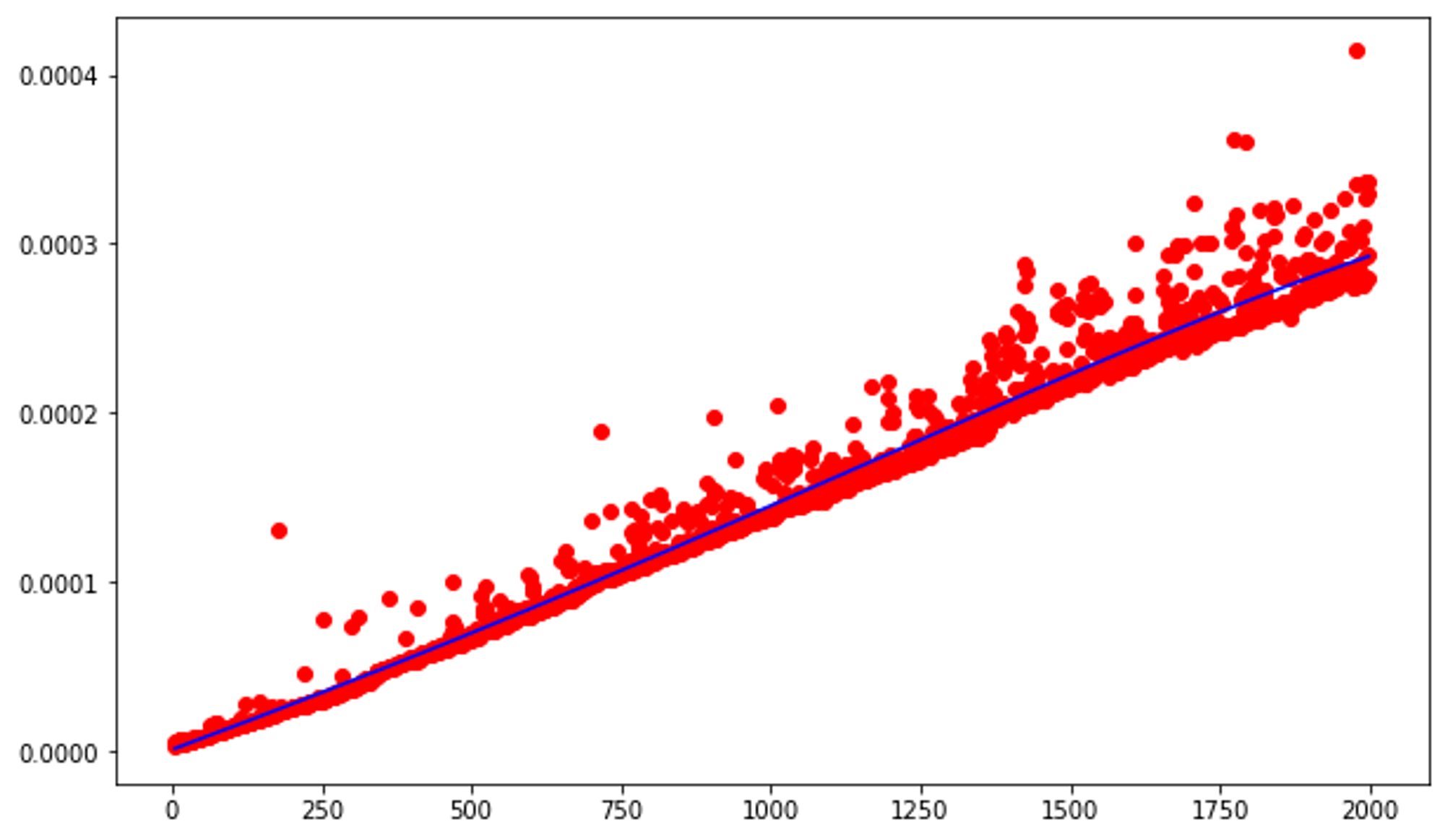
Without even comparing this graph to the graphs of the possible runtimes, we can already safely assume that this function operates in O(n) runtime.
Mystery function #2
1
2
3
4
5
6
7
8
9
10
11
12
13
14
15
16
17
18
19
20
def g(l): # l is a python list of integers of length n
  pairs = [ (i,j) for i in range(len(l)) for j in range(len(l)) if i < j ]
  result = []
  for (i,j) in pairs:
    if l[i] == l[j]:
      result.append((i,j))
  return result

ns = range(5, 200)
ts = [timeit.timeit('g(lst)',
                    setup='lst=list(range({}))'.format(n),
                    globals=globals(),
                    number=1)
         for n in ns]
plt.plot(ns, ts, 'or')

degree = 4
coeffs = np.polyfit(ns, ts, degree)
p = np.poly1d(coeffs)
plt.plot(ns, [p(n) for n in ns], '-b')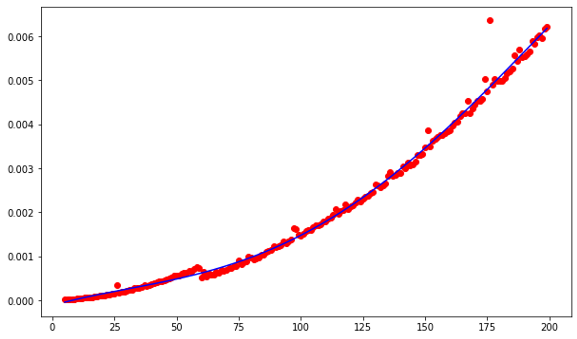
This graph looks very similar to the one for insertion sort, so we can determine that this function has a runtime complexity of O(n^2).
Mystery function #3
1
2
3
4
5
6
7
8
9
10
11
12
def h(n):
   if n <= 1:
       return n
   else:
       return h(n-1) + h(n-2)

ns = range(5, 30)
ts = [timeit.timeit('h({})'.format(n),
                    globals=globals(),
                    number=1)
         for n in ns]
plt.plot(ns, ts, 'or')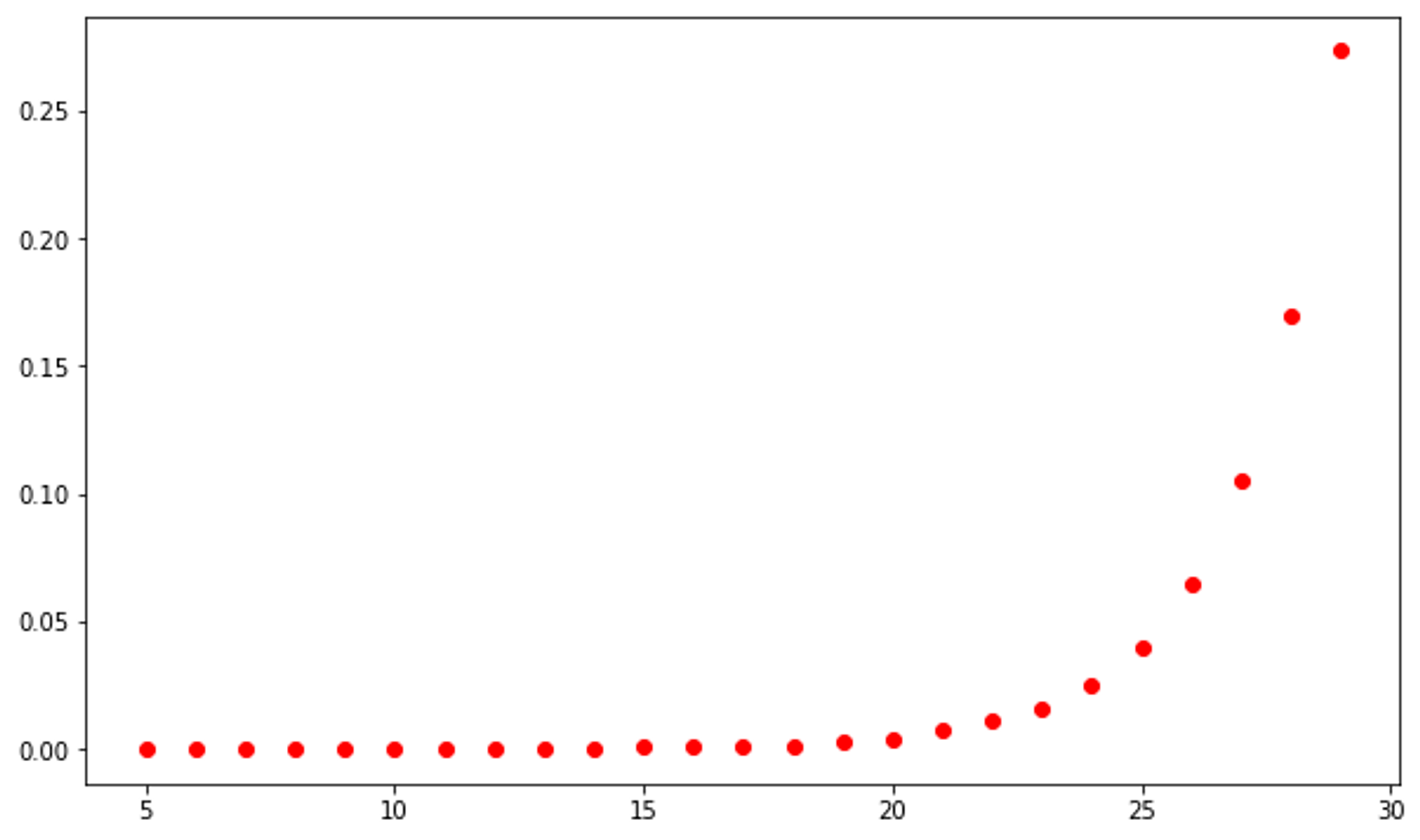
This function is more ambiguous than the previous two. It is evident that its runtime must be greater than O(n) as the slope increases as n increases. Let's consider the graphs of runtimes O(n^2) in red and O(2^n) in blue.
1
2
3
4
5
6
7
8
9
10
11
# y = n^2
# vertically stretched 20x
ns = range(5, 30)
ts = [n*n*20000 for n in ns]
plt.plot(ns, ts, 'or')

# y = 2^n
# vertically compressed 50x
ns = range(5, 30)
ts = [math.pow(2, n)/50 for n in ns]
plt.plot(ns, ts, 'ob')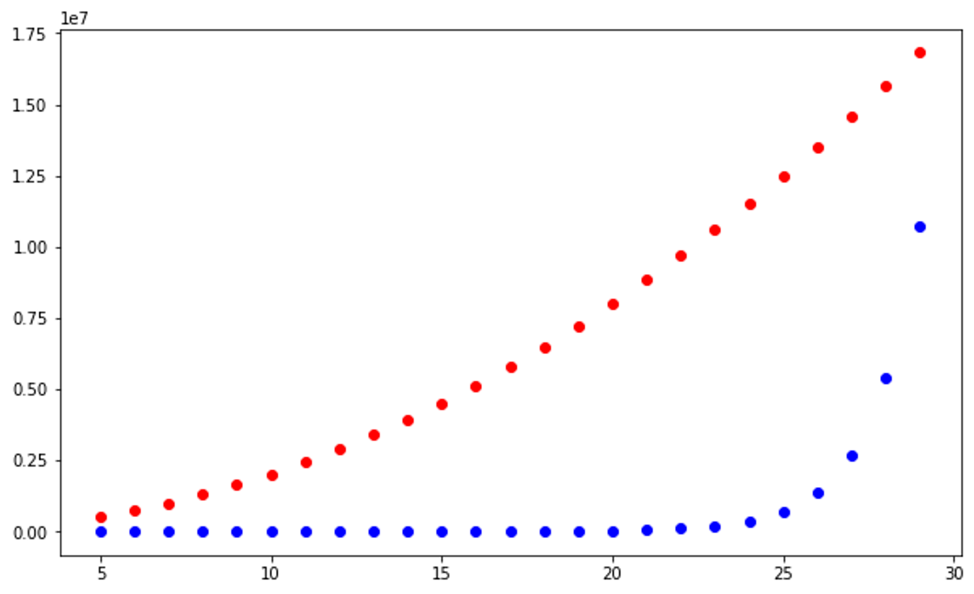
The graph of the runtime of mystery function #3 more closely resembles the blue plots, so therefore the runtime complexity of mystery function #3 is O(2^n).
Conclusion
Using these visualization libraries, we are able to determine the runtime complexities of functions and algorithms by comparing them to plots/graphs of known runtimes (i.e. comparing plots of insertion sort runtime against y=n^2). In addition to determining runtime complexities, this methodology can be used to compare the speeds of different algorithms against each other. With only a few lines of code, you can quickly see the speed at which your chosen algorithms will run with large sets of data.
Subscribe to Instructive.dev
Don’t miss out on the latest content! Join over 3k+ devs in subscribing to Instructive.dev.
Join the mailing list